Undergraduate Thesis · Computer Vision
How do CNNs and Vision Transformers actually arrive at a diagnosis?
Benchmarking Vision Transformers Against CNNs for Plant Disease Diagnosis: Performance, Robustness, and Visual Interpretability
- YOLO leaf localization
- Species classifier
- ResNet-50 vs. ViT-B/16
- Grad-CAM · attention rollout
Where it started
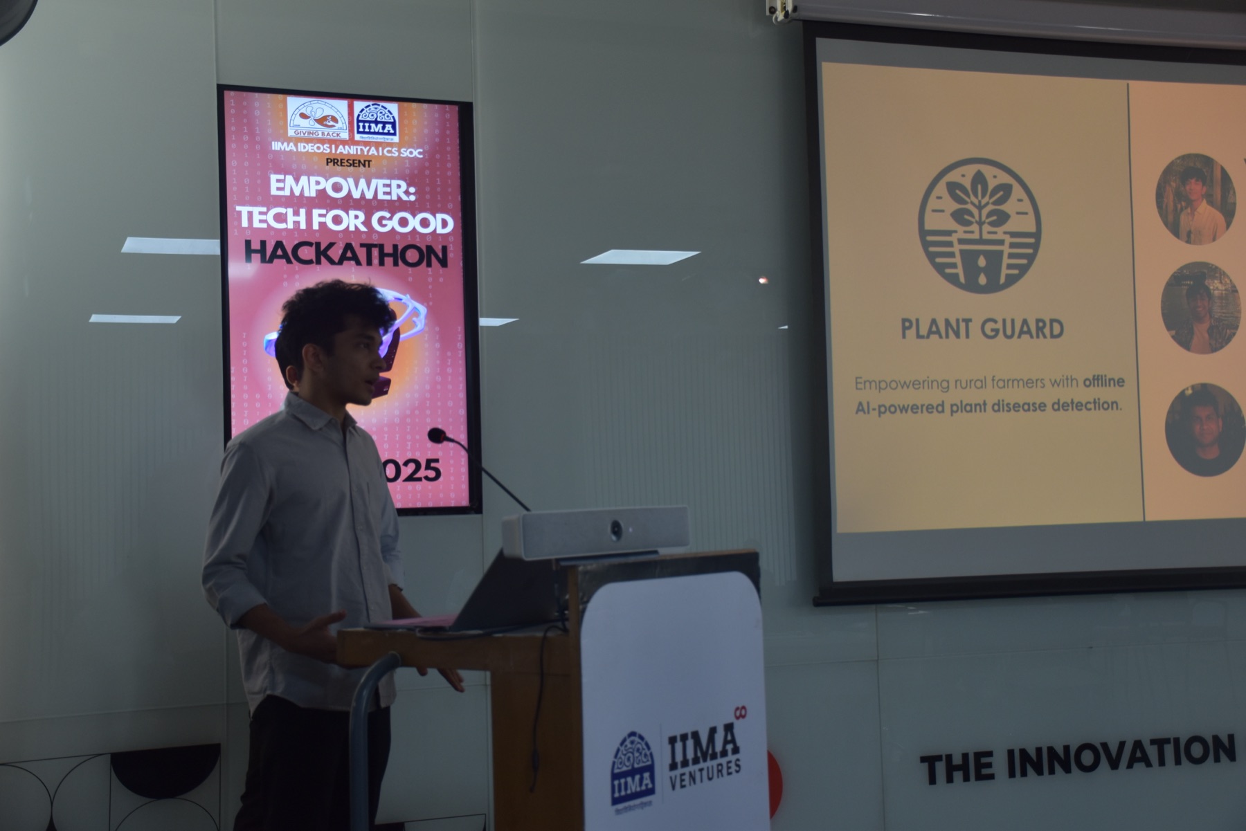
This thesis started as PlantGuard: an offline, AI-powered plant disease detector that my team built for the EMPOWER hackathon, and which went on to win it in 2025.
PlantGuard needed models that worked. The thesis asked a slower question about those same models: when a CNN and a Vision Transformer both get the diagnosis right, are they looking at the same thing?
The question
Comparisons between CNNs and Vision Transformers usually stop at accuracy: whichever scores higher wins. But two architectures can reach the same number while relying on completely different visual cues, and that difference shows up later as differences in robustness, interpretability and failure modes.
The thesis asks two questions:
- RQ1: Do Vision Transformers outperform CNNs under controlled, identical conditions?
- RQ2: How does each architecture’s inductive bias show up in the features it actually uses?
A pipeline built for a fair comparison
Disease labels only make sense for a given species, and end-to-end models tend to pick up backgrounds and cross-species shortcuts. So the task is decomposed the way an agronomist would approach it: find the leaf, identify the species, then predict the disease from a label space restricted to that species.
The decomposition does double duty. It is a better system design, and it is also the experimental control: by standardizing everything upstream, the only thing that changes between runs is the classifier architecture.
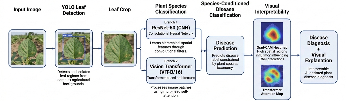
About 54,000 images across 13 species and 38 classes (including healthy), split 80:10:10, with rotation, flip and color-jitter augmentation. Both models start from ImageNet weights and train in PyTorch on an NVIDIA A100. The YOLO stage reached mAP@0.5 of 0.93 (precision 0.90, recall 0.88), so the classifiers were seeing clean leaf crops.
Training settings are shared except where the inductive bias justifies a difference: the ViT gets a lower learning rate (5e-5 vs. 2e-4), warmup with cosine annealing, label smoothing, dropout and much stronger weight decay to make up for the implicit regularization a CNN gets from weight sharing.
Accuracy: a small gap
| Stage | ResNet-50 | ViT-B/16 |
|---|---|---|
| Species classification | 96.2% | 96.8% |
| Disease classification | 92.7% | 93.8% |
| End-to-end pipeline | 89.4% | 90.6% |
The ViT wins everywhere, but only by about a point. That is exactly the regime where the interesting question isn’t which model is better, but whether they are solving the problem the same way.
The trade-offs also follow the theory: the CNN stayed stable across learning rates and ran faster at inference, while the ViT reached a higher peak only when tuned carefully, and paid for global self-attention in compute.
Same leaf, different evidence
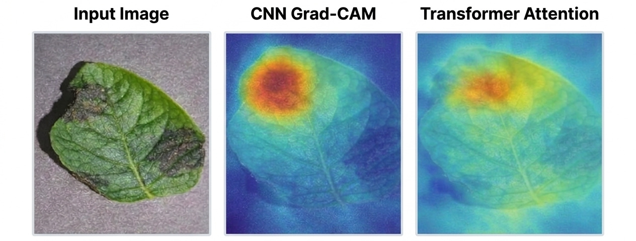
To get past eyeballing heatmaps, I compared Grad-CAM maps from the CNN with attention-rollout maps from the ViT across 1,100 test images, using three metrics.
| Metric | ResNet-50 | ViT-B/16 | Reading |
|---|---|---|---|
| Saliency entropy (nats) | 3.84 ± 0.41 | 5.67 ± 0.38 | ViT is 1.83 nats more diffuse (p < 0.001) |
| Top-10% mass concentration | 0.713 | 0.487 | CNN concentrates far more energy in few pixels |
| Lesion overlap (IoU) | 0.61 | 0.44 | CNN aligns more closely with visible lesions |
Lower lesion overlap doesn’t mean the ViT is looking at the wrong thing. It is using context outside the lesion boundary, like vein structure, color gradients and how symptoms are distributed across the leaf, that is still diagnostically relevant.
These maps are correlational, not causal explanations, so the claims are comparative. But the divergence is consistent across the test set, which points to a systematic effect of architecture rather than a few cherry-picked examples.
Each model fails in character
The failure modes line up with each architecture’s bias, which is part of the evidence that they are structural rather than incidental.
- ResNet-50: background texture bias, sensitivity to lighting, and confusion between diseases with similar local texture.
- ViT-B/16: missing fine-grained local detail, especially in early-stage disease where the signal is concentrated in a small area, and occasionally smoothing attention over irrelevant regions.
- Both: visually similar disease classes, and early-stage disease misread as healthy.
The practical reading: when symptoms are localized and the images are high-resolution, a CNN may be the more reliable choice. When the cues are spread across the leaf, or robustness to local noise matters, a ViT is the better bet.
What I took from it
Architecture doesn’t only decide how accurate a model is. It decides what kind of reasoning the model does. Two models within a point of each other on the test set can behave very differently under distribution shift, perturbation or deployment, and accuracy alone hides that.
Limitations
- The images come from controlled or semi-controlled conditions, not messy field deployments.
- Grad-CAM and attention maps are approximate indicators, not ground-truth explanations.
- No formal robustness guarantees or analysis of decision-boundary geometry.
- Errors compound across the pipeline stages, and that propagation isn’t formally analyzed.
Where it goes next
- Hybrid CNN–ViT architectures that fuse local precision with global reasoning.
- Robustness as a training objective: adversarial augmentation, domain randomization, field data.
- Causal interpretability: counterfactual explanations and feature ablations instead of heatmaps alone.
- Edge deployment of ViTs through quantization, pruning and distillation.
- Theory: representation geometry and optimization dynamics behind the behavioral differences.
Evidence
- ViT-B/16 beat ResNet-50 at every stage: 93.8% vs. 92.7% on disease classification, 90.6% vs. 89.4% end to end.
- ViT attribution maps were 1.83 nats more diffuse (saliency entropy 5.67 vs. 3.84, p < 0.001, n = 1,100).
- The CNN put 71% of its attribution mass in the top 10% of pixels, against 49% for the ViT, and overlapped lesions more (IoU 0.61 vs. 0.44).